Linear programming calculator: solve LP problems step by step

You probably landed here for one of two reasons: you have an optimization problem to solve right now, or you want to understand what a linear programming calculator is doing before you trust the number it gives back. This guide handles both, with worked examples you can follow and check by hand.

Linear programming turns up in a lot of ordinary situations. A workshop deciding how many tables and chairs to build. A nutritionist mixing feed at the lowest cost. A student grinding through an operations research assignment. A good LP calculator answers these in seconds, but the setup is where people trip, and a wrong setup gives a confident wrong answer. So the plan is simple: understand the parts, feed the calculator correctly, then verify what it hands back.

What a linear programming calculator does

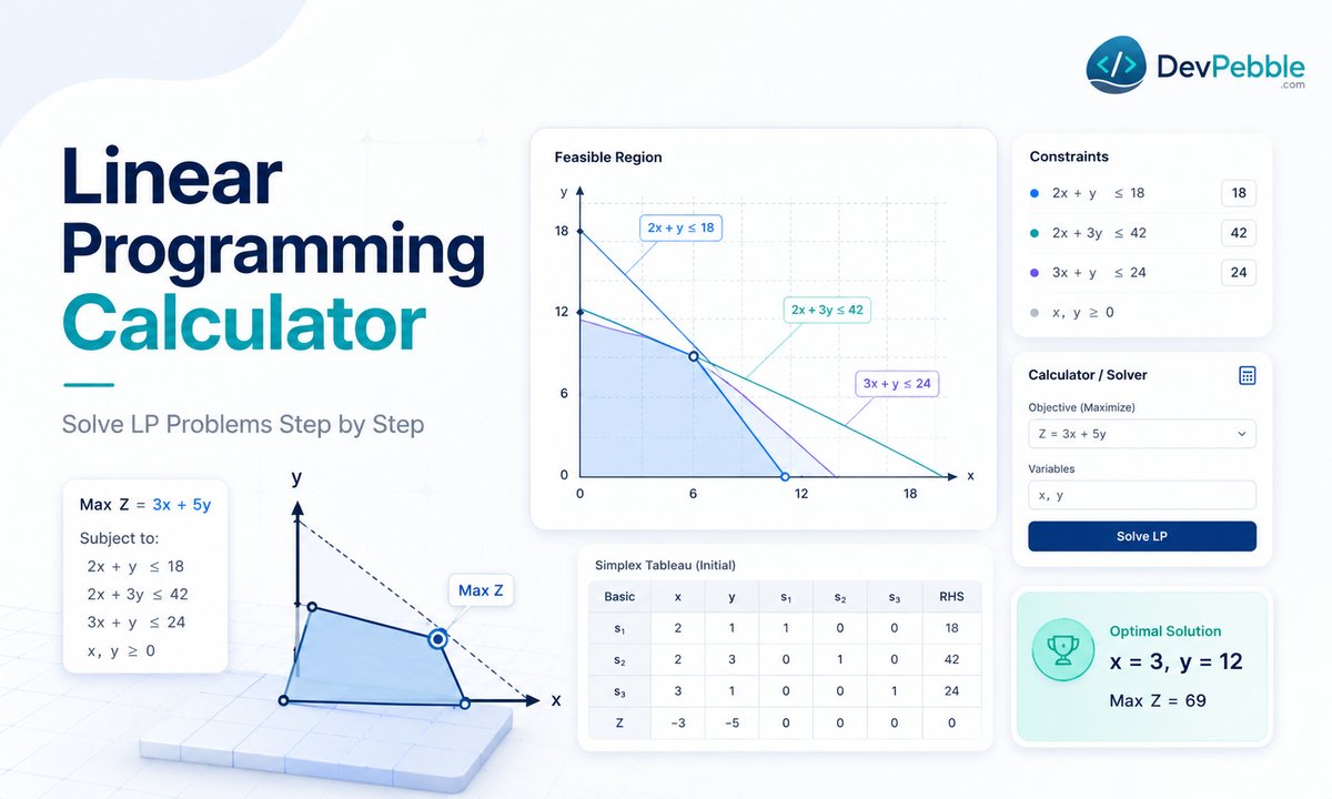
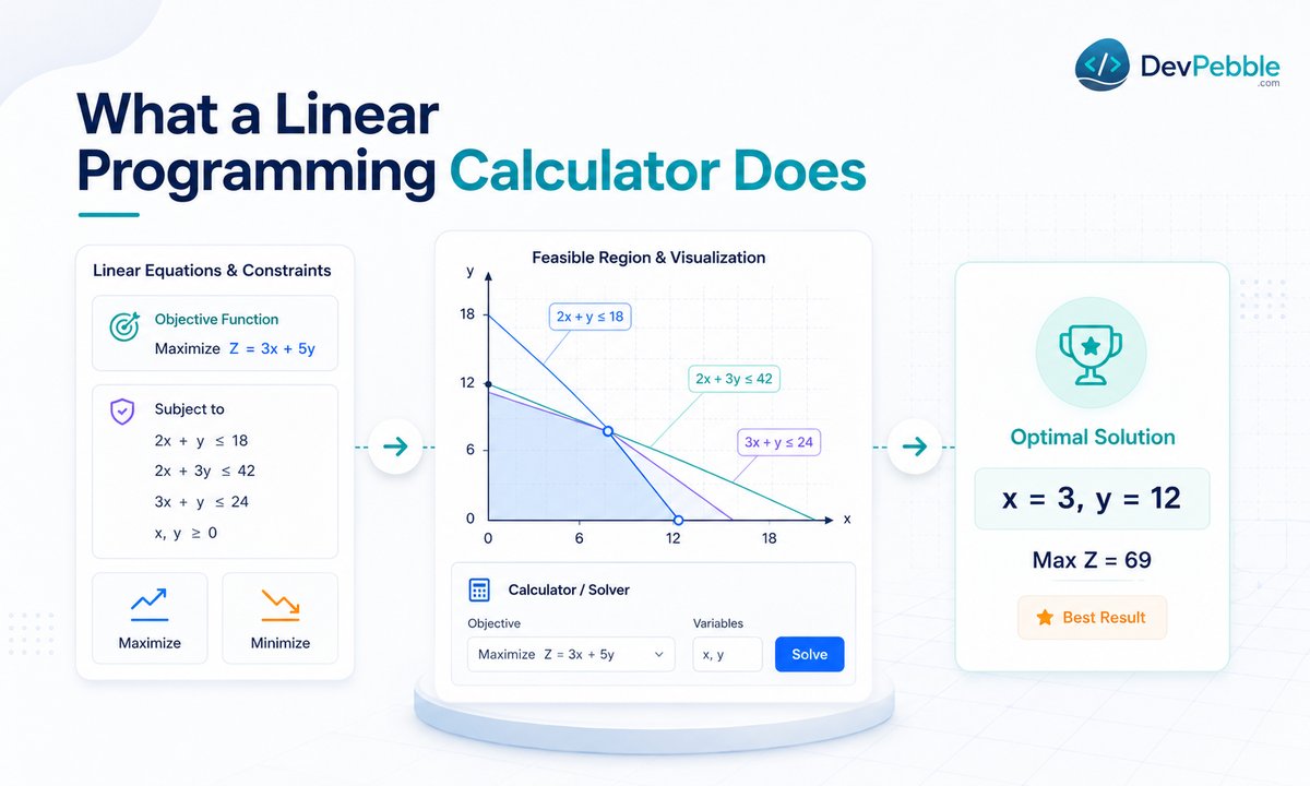
A linear programming calculator (you will also see it called an LP solver) finds the best possible outcome for a problem where you want to push some quantity as high or as low as it will go, inside a fixed set of limits. You type in a goal and a list of restrictions, and it runs the math for you, usually with the graphical method for two variables or the simplex method for anything bigger.

It only works when the relationships are linear, meaning everything scales in straight lines with no exponents or variables multiplied together. Within that limit, it covers a wide range of everyday problems: squeezing the most profit out of limited materials and labor, hitting a production target at the lowest cost, splitting a budget across channels for the best return, or building a staff schedule that meets demand without overspending.

You do not need a maths degree to use one. Students in operations research or business courses lean on them, and so do managers sizing up production runs, analysts who want a fast answer without building a spreadsheet model. If you have a clear goal and limited resources, the problem is probably a linear programming problem, and a calculator can solve it.

The three parts of every LP problem

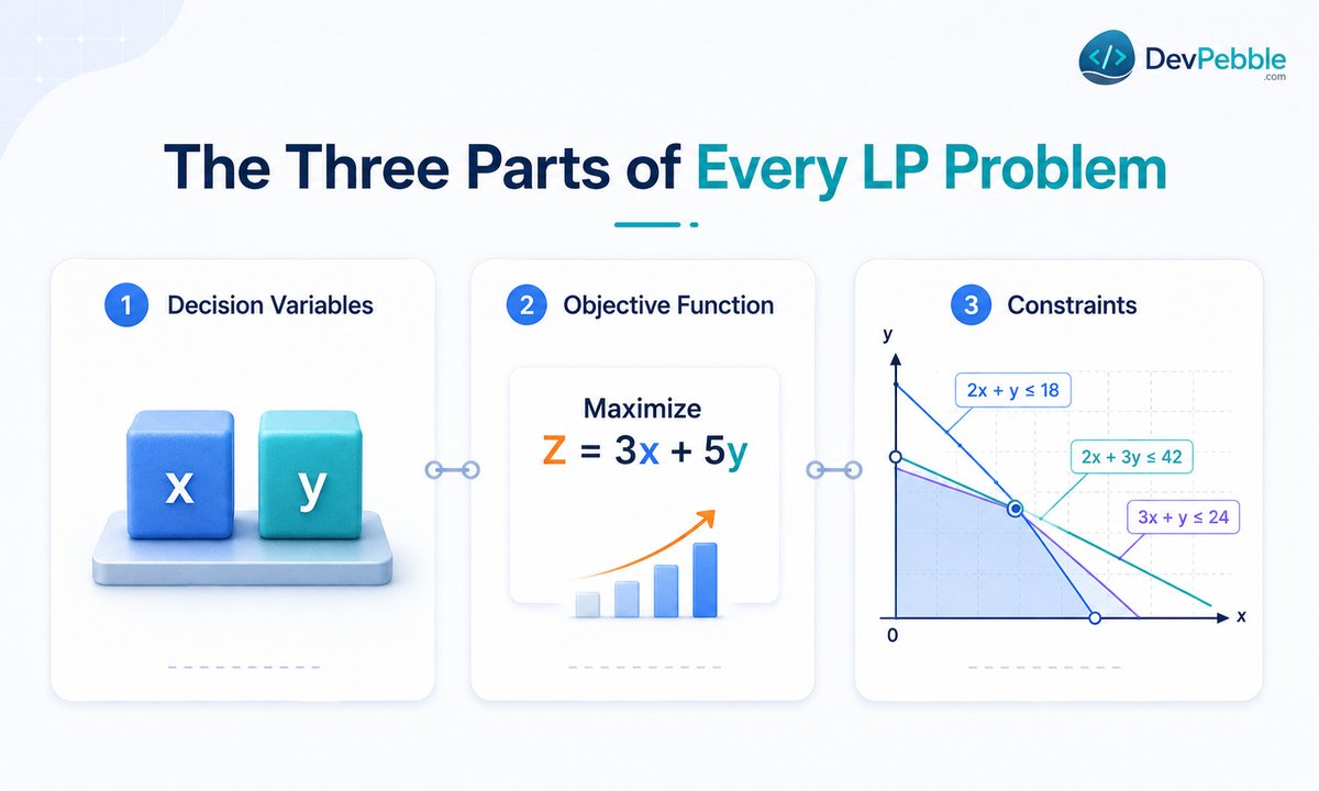
Before typing anything, it helps to see the three pieces in every linear programming problem. Once these make sense, the calculator fields stop looking cryptic.

Decision variables

Decision variables are the unknowns you control. Take a small furniture workshop that makes tables and chairs. You would let x be the number of tables and y the number of chairs. The whole job of the solver is to find the best values for x and y.

The objective function

The objective function is the goal, written as a single equation to maximize or minimize. If each table earns $50 profit and each chair earns $30, the profit goal is Z = 50x + 30y, and you want it as high as possible. That one line tells the calculator what a good answer looks like.

Constraints and the feasible region

Constraints are the real limits that stop your variables from running off to infinity, usually tied to time, money, materials, or labor. For the workshop, they might be 2x + y ≤ 40 (machine hours) and x + 3y ≤ 30 (labor hours). You almost always add non-negativity conditions too, x ≥ 0 and y ≥ 0, because you cannot build a negative chair.

Together the constraints carve out a feasible region, the set of all solutions that break no rules. One fact does most of the heavy lifting in linear programming: the best answer always sits at a corner of that region, never floating somewhere in the middle. Solvers take advantage of this by checking corners instead of the infinite points inside.

What a linear programming calculator asks you for

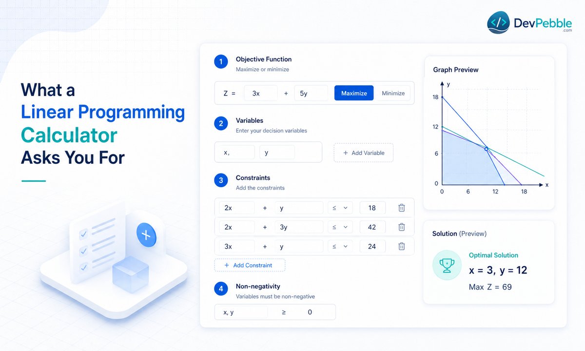
Most calculators want the same three things, in the same order.

First, whether you are maximizing or minimizing. Profit, output, and return get maximized. Cost, waste, and time get minimized. This flips how the solver searches, so it matters.

Second, the objective function coefficients, which are just the numbers attached to each variable. In the furniture example those are 50 and 30. They tell the tool how much each table and chair adds to the total.

Third, the constraints, entered one inequality at a time with their limits. Most tools let you add as many as you need, and many switch on the non-negativity conditions for you. Confirm that they did, because a missing constraint is the quickest route to a wrong answer. With those three in place, the calculator has what it needs.

How to use a linear programming calculator step by step

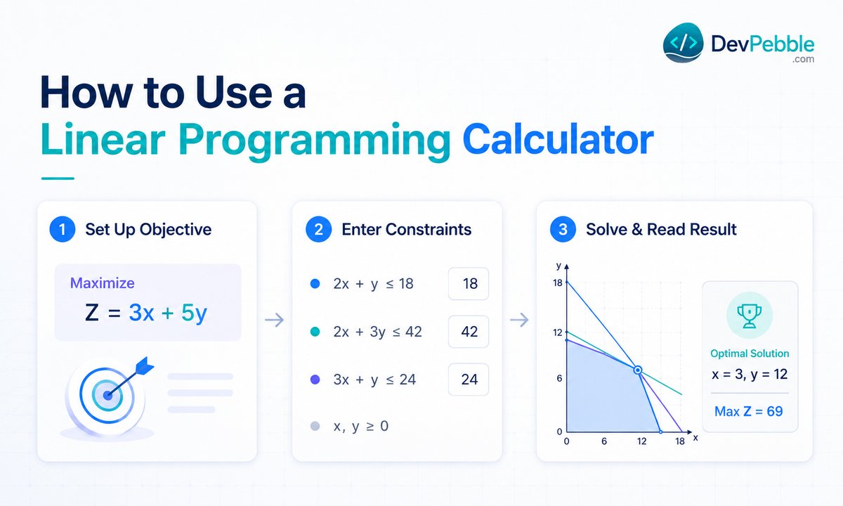
Step 1: Set up the objective function

Write out what you are optimizing in the form Z = (number times variable) + (number times variable). For the workshop that is Z = 50x + 30y, with x for tables and y for chairs. Choose maximize or minimize first, then drop in the coefficients. One thing worth checking before you commit: your units. Mixing hours with days, or dollars with hundreds of dollars, is one of the most common setup slips.

Step 2: Enter every constraint

Give every resource limit its own line: machine hours, labor, budget, materials, each as a separate inequality.

• 2x + y ≤ 40
• x + 3y ≤ 30
• x ≥ 0, y ≥ 0

Most calculators add the non-negativity lines for you, but a quick glance to confirm beats debugging a strange result later.

Step 3: Solve and read the result

Hit solve. A decent solver returns three things: the best value for each variable, the best value of the objective, and often the exact corner of the feasible region where that happens. Do not just read the final number. The variable values are the real decision; the objective only tells you how good it is.

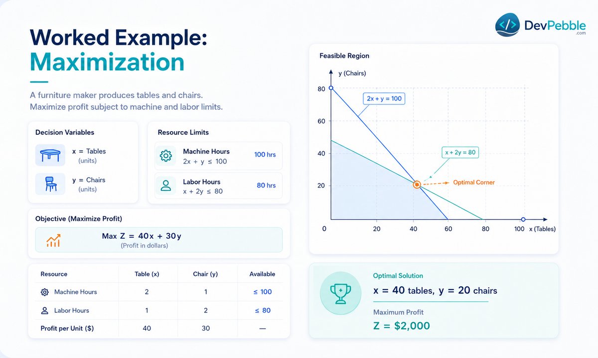
Worked example: a maximization problem

The setup

A workshop builds tables and chairs. Each table earns $50 profit, each chair $30. A table needs 2 hours of machine time and 1 of labor; a chair needs 1 hour of machine time and 3 of labor. There are 40 machine hours and 30 labor hours available. That gives:

• Maximize Z = 50x + 30y
• 2x + y ≤ 40
• x + 3y ≤ 30
• x, y ≥ 0

Reading the calculator output

Run it and you get x = 18, y = 4, with a maximum profit of Z = $1,020. In plain terms, build 18 tables and 4 chairs. Many calculators also flag which constraints are binding (fully used) versus which have slack left over. Here both are binding, so every machine and labor hour is spent at the optimum.

Checking the answer

Plug the numbers back into the original limits:

• 2(18) + 4 = 40 ✓
• 18 + 3(4) = 30 ✓

Both hold exactly, which confirms the solution is valid. If a calculator ever hands you numbers that break a constraint, that is a typo in your setup, not a failure of the method.

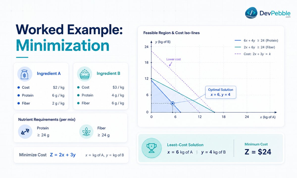
Worked example: a minimization problem

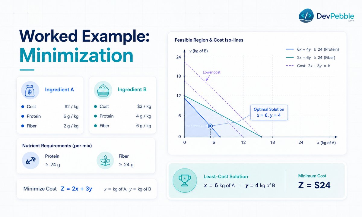
Minimization runs the same way with the goal flipped, and it usually brings ≥ constraints instead of ≤.

Say a company blends two ingredients, A and B, into animal feed. A costs $4 per unit, B costs $6. The feed needs at least 20 units of protein and 30 units of fiber. Each unit of A supplies 2 protein and 3 fiber; each unit of B supplies 4 protein and 2 fiber. The problem becomes:

• Minimize Z = 4x + 6y
• 2x + 4y ≥ 20 (protein)
• 3x + 2y ≥ 30 (fiber)
• x, y ≥ 0

The ≥ signs are the tell: you are meeting minimums, not staying under caps. Solved, this one lands at x = 10, y = 0, for a cost of Z = $40, so 10 units of A and none of B. Both the protein and fiber requirements come out exactly met at that point, so both constraints are binding.

When a requirement ends up with room to spare (protein above the required 20, say), that constraint is non-binding: it was not the thing holding the solution back. Knowing which constraints bind tells you where your real bottleneck is, often more useful than the cost figure itself.

The graphical method for two-variable problems

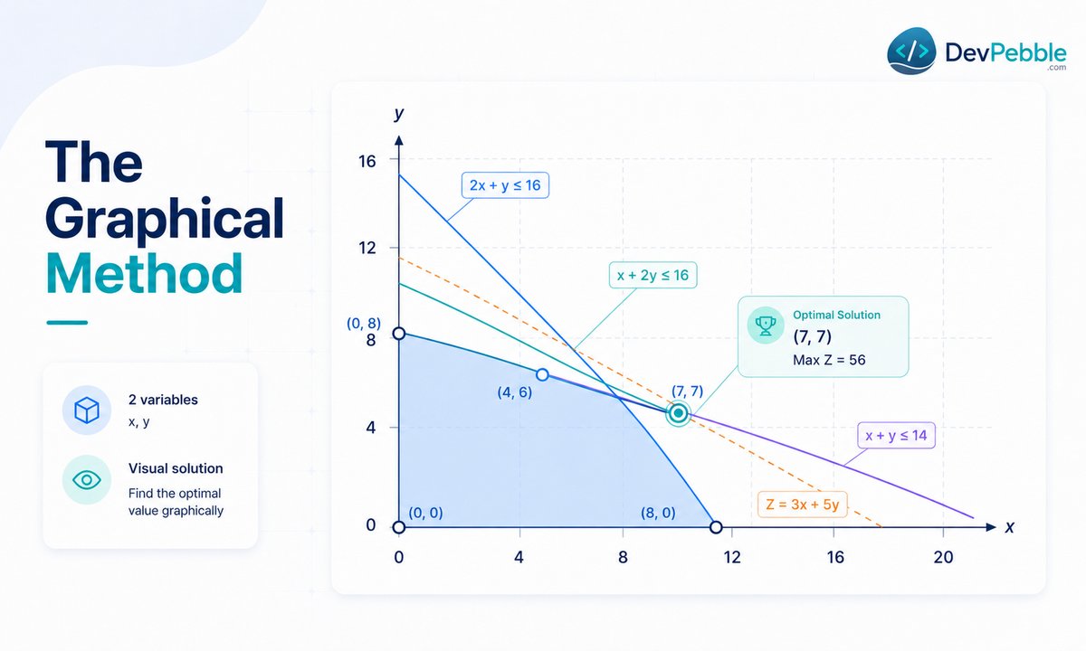
With only two variables, a graphical method calculator is the easiest way to see what is going on. Each constraint becomes a line on an x-y plane, and the feasible region is the overlapping area that satisfies all of them at once, essentially the zone where your answer is allowed to live.

The optimum always lands on a corner of that region. A graphical calculator finds every corner, tests the objective at each one, and reports the best result. It is great for learning and for simple problems, but it falls apart the moment you add a third variable, since you cannot easily picture a feasible region in three dimensions. That is where the simplex method takes over.

The simplex method for larger problems

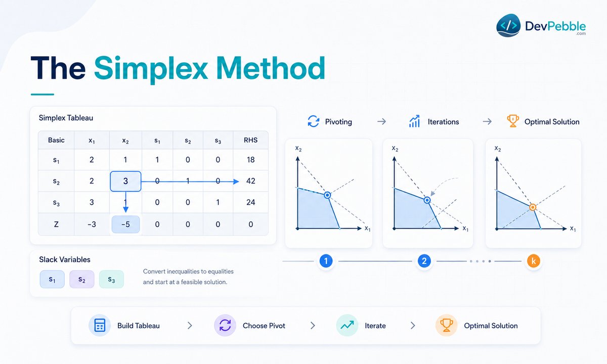
For more than two variables, a simplex calculator works through the problem algebraically instead of drawing it.

Slack, surplus, and artificial variables

The method first turns inequalities into equations by adding helper variables. Slack variables get added to ≤ constraints, surplus variables get subtracted from ≥ constraints, and artificial variables are sometimes added on a temporary basis to get ≥ or = constraints started. None of these represent real decisions. They are bookkeeping that makes the algebra work.

Pivoting and iterations

Everything goes into a grid called a simplex tableau. The method picks a pivot column (typically the most negative entry in the objective row) and a pivot row (from the smallest ratio test), then rewrites the whole tableau. Each pass is an iteration, and it repeats until no move improves the objective. The final tableau reads out the optimal variable values and objective, the same answer the graphical method would give, reached a different way. Most online tools do all of this silently, but seeing the tableau helps you trust the output instead of treating it as a black box.

Big M, two-phase, and dual simplex

Some problems will not start cleanly under plain simplex, usually the ones with ≥ or = constraints and no obvious feasible starting point. A few variations exist for exactly this. The Big M method puts a large penalty on artificial variables so the solver drives them out fast. The two-phase method solves a smaller warm-up problem first to find a feasible starting point, then tackles the real objective. Dual simplex is handy when a solution is optimal but not yet feasible, which often happens after you tweak a problem you already solved. You will rarely run these by hand. Most calculators offer them as a setting, and knowing what each one is for explains why a tool might reach for something other than plain simplex.

Integer programming when fractions do not work

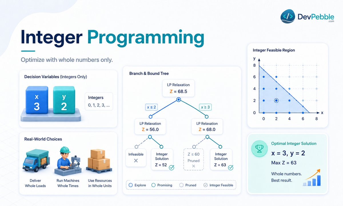
Not every problem accepts fractional answers. If you are deciding how many delivery trucks to buy, 4.7 trucks is useless. An integer linear programming calculator restricts some or all variables to whole numbers, which matters for anything counted in people, vehicles, or machines.

Most of these solvers use branch and bound. The solver first ignores the whole-number rule and solves it as an ordinary LP. If the answer comes back with fractions, it splits into two smaller problems (rounding a variable up in one, down in the other) and keeps branching until it finds the best whole-number solution that still obeys every constraint. It sounds heavy, but the calculator handles it in the background.

How to check a calculator answer and avoid common mistakes

Even a solid solver only reflects the inputs you gave it. Most wrong answers trace back to setup, not the tool, and a one-minute check catches almost all of them.

Start by plugging your solution into every constraint. Each inequality should hold; if one is violated, something was entered wrong even if the tool raised no error. Then recompute the objective by hand, multiplying each variable by its coefficient. If that does not match the tool's value, it read your goal incorrectly.

A few setup mistakes come up again and again. Mixing up ≤ and ≥ is the big one: a resource cap should almost always be ≤, while a minimum requirement like protein or staffing should be ≥. Forgetting the non-negativity lines can produce nonsense like negative production, so confirm they are on. And check that your goal matches the problem, since selecting maximize on a cost problem inverts the entire logic.

Sometimes the calculator returns no numbers at all, just a note that the problem is infeasible or unbounded. Those are real answers, not errors. Infeasible means no point satisfies every constraint at once, so the constraints contradict each other. Unbounded means the objective can improve forever, almost always because a constraint is missing.

What to look for in a good calculator

Calculators vary more than you would expect. A good one shows its work, whether that is the simplex tableau iterations or the graphical corner points, so you can learn from it rather than copy a number. For two-variable problems, a plotted feasible region with the optimal point marked makes the answer click. And support for simplex, Big M, two-phase, and integer constraints means you will not have to switch tools as your problems get harder.

Online calculator vs Excel Solver vs Python

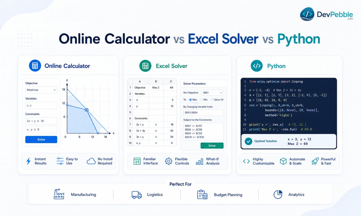
Which tool fits depends on the job.

For quick problems, homework, or testing an idea, an online linear programming calculator is usually fastest. No setup, instant results.

If your data already lives in a spreadsheet, Excel Solver is the practical pick. It suits business tasks like budgeting or scheduling, where you want the model wired directly to your existing numbers.

For larger, repeatable, or automated work, Python tools give you far more control. SciPy's linprog function now runs on the HiGHS solver by default and handles sizeable problems well, while Google's OR-Tools (with its Glop solver) scales to serious optimization across Python, C++, Java, and C#. These suit developers wiring optimization into a system, not one-off calculations.

Where linear programming gets used

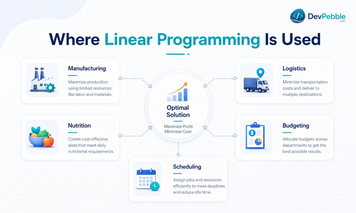
The same math shows up across very different fields. Manufacturers use it to decide how much of each product to run given limited machine time, labor, and materials. Nutritionists and food producers use it to meet dietary requirements at the lowest ingredient cost. Logistics teams use it to cut shipping costs across routes or to schedule staff against demand. Plenty of businesses use it to split a limited budget across projects for the best return. If a decision involves scarce resources and a measurable goal, linear programming can usually model it.

Final thoughts

A linear programming calculator saves time and cuts down on arithmetic errors, but it is only as good as the problem you hand it. The real skill is not clicking solve. It is setting up the objective, entering constraints with the right inequality signs, and reading the result, including what infeasible and unbounded are telling you. Get that right and the calculator stops being a black box and becomes a decision tool you can trust. When in doubt, spend the extra minute to check by hand. It is the cheapest insurance in the process.